
Sports Coupe Aerodynamic Performance Analysis
At a configured 120 km/h, full-vehicle streamlines, velocity sections and load statistics connect body flow and wake deficits with drag and vertical-load variation.
00 / Connect shape observations with comparable metrics
Engineering question
Coupe aerodynamics involves both resistance to motion and vertical loading. The nose, roof, underbody and wheel regions redirect the incoming flow, while the rear geometry influences how those streams merge into a wake. A streamlined appearance alone cannot establish the integrated loads or identify which regions will respond most strongly to a local geometry change.
This study reads global streamlines, two velocity-section orientations and late-window load statistics together. The flow views locate regions of interest; the loads quantify the integrated response. The aim is to establish a baseline for geometry comparisons and identify the evidence still needed, rather than rank shapes from a single contour image.
At the 120 km/h baseline condition, what are the drag and vertical loads, and which flow regions deserve the next design investigation?
- configured freestream speed
- 120 km/h
- mean aerodynamic drag
- 561.03 N
- mean drag coefficient
- 0.4442
- samples in the statistics window
- 4,575
01 / Establish conditions, reference quantities and sampling
A straight-ahead baseline at 120 km/h
The current configuration specifies zero angle of attack and sideslip, with an air density of approximately 1.225 kg/m³. Its Mach number is about 0.098 and its 4.2341 m reference length gives a Reynolds number of approximately 9.66×10⁶. The analysis uses incompressible unsteady external-flow evidence under the conditions below.
- Freestream speed
- 120 km/h (33.33 m/s)
- Incidence / sideslip
- 0° / 0°
- Air density
- 1.225 kg/m³
- Reference area / length
- 1.8559 m² / 4.2341 m
- Configured Ma / Re
- 0.098 / 9.66×10⁶
- Statistics window
- Final 25% · 4,575 samples
Reference area affects coefficient normalization. Compare force values and coefficients together so a changed reference quantity is not mistaken for better performance. Moving-ground and wheel-rotation settings have not been fully confirmed in the available material. Their influence on underbody and wheel-region flow requires consistent-condition checks; road-equivalent boundaries cannot be assumed.
02 / Relate global paths to local velocity distributions
Roof acceleration, wheel disturbances and a wake deficit
Use the full-vehicle streamlines to establish spatial relationships, then inspect the scaled sections for velocity changes. These views represent the selected exported flow field, not an established average over the load-statistics window. Mean-load conclusions rely on the separate load statistics.
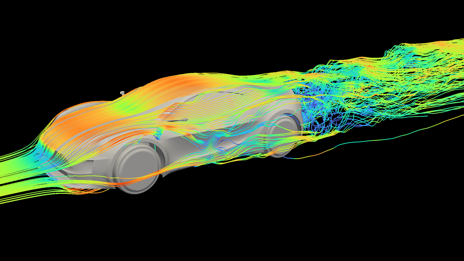
Full-vehicle streamlines show flow dividing around the nose, roof and sides, then merging and bending behind the rear body. Color represents velocity magnitude, but this rendering has no readable quantitative scale, so it supports inspection of paths and local structures. A streamline represents direction in the selected flow field; this static image does not establish shedding frequency or a local drag contribution.
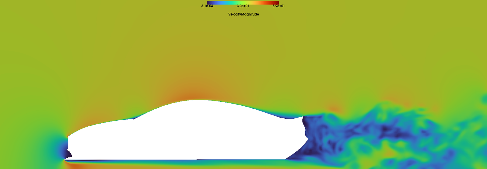
The longitudinal section uses velocity magnitude in m/s. Higher speeds occur near the roof, with a continuous low-speed region behind the vehicle and a distinct underbody path. Local acceleration and the downstream momentum deficit therefore need to be assessed together. Velocity magnitude alone does not determine reverse flow; inspect vectors or the streamwise velocity component before identifying recirculation.
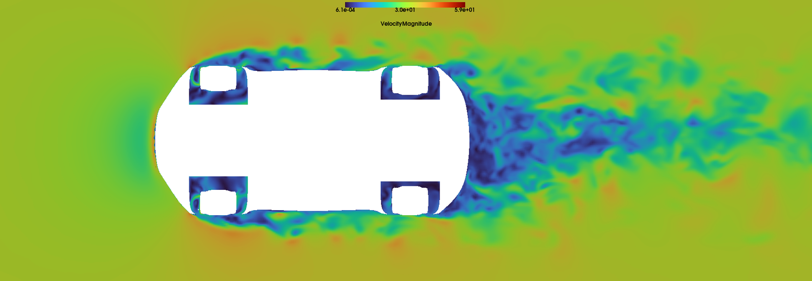
The horizontal section shows nonuniform velocity around the wheels and along the body sides, connecting those disturbances to the rear wake. A wheel-region or side-body change may therefore affect downstream flow as well as the local field. Compare designs at the same section position, color range and sampling convention to examine the extent and recovery of the low-speed region.
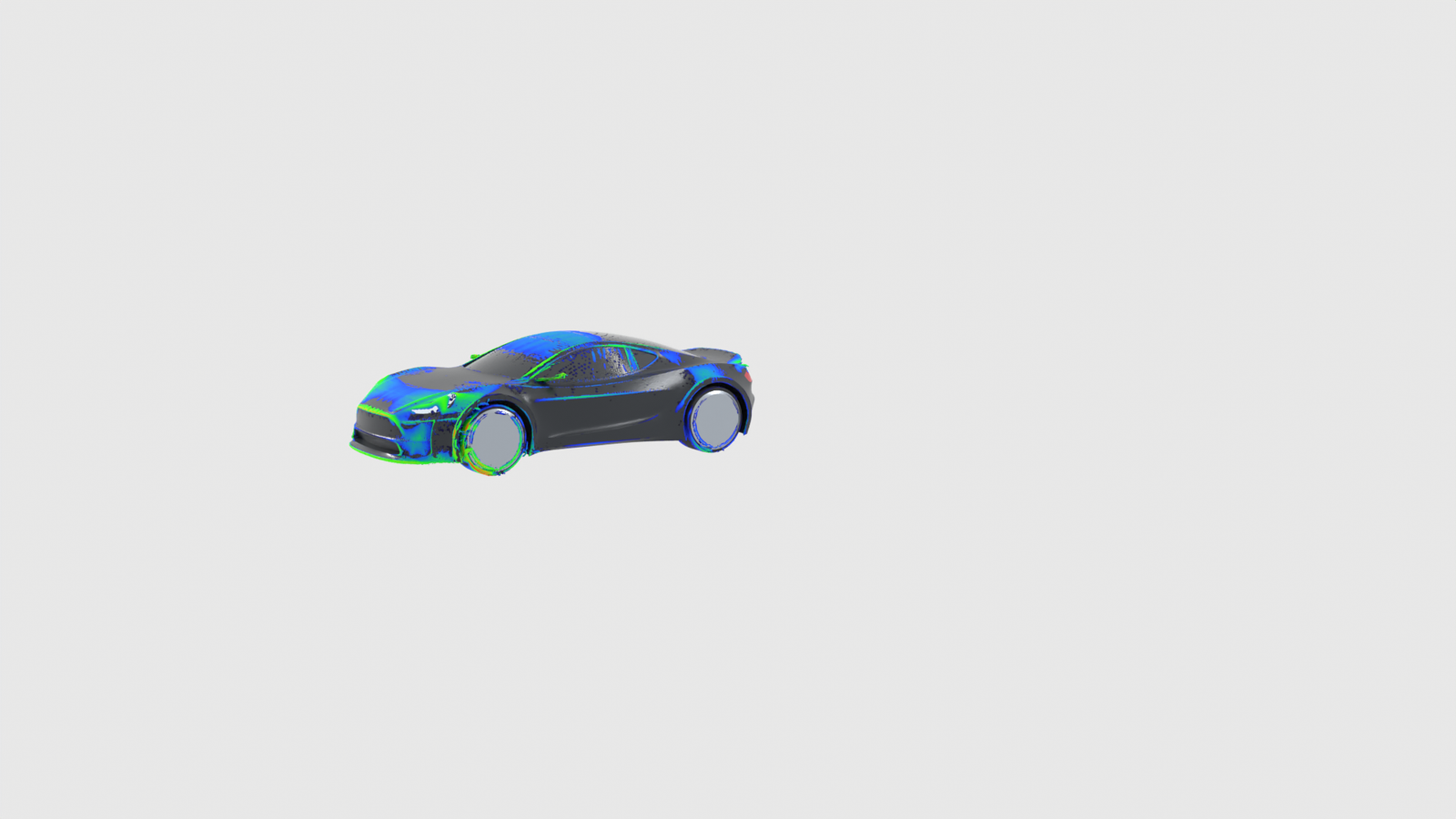
The Q-criterion isosurface highlights local rotating structures near body edges and wheel regions. It helps locate areas for closer inspection, but its appearance depends on the threshold and sampling instant. This rendering does not decompose aerodynamic loads; component drag requires pressure and viscous-force integration over the relevant surfaces.
Questions the flow evidence can help test
- 01Does a rear transition change consistently alter the low-speed region and its recovery? Compare matched sections and pressure recovery, not colors alone.
- 02Do wheel-region and side-body changes affect the downstream wake and integrated drag together? A more orderly local image does not automatically imply lower total drag.
- 03Does an underbody change trade drag against lift or pitching moment? Evaluate the benefit against all relevant load metrics.
03 / Quantify the integrated response with load statistics
Drag sets a power scale; lift needs a fluctuation check
Mean drag in the final statistics window is 561.03 N. Its fluctuation RMS is 17.87 N, approximately 3.19% of the mean. The mean drag coefficient is 0.4442, reported as exported for this baseline. It is not a direct ranking across vehicles or reference-area conventions.
| Load | Mean / N | Fluctuation RMS / N | Mean coefficient |
|---|---|---|---|
| Drag | 561.03 | 17.87 | Cd = 0.4442 |
| Lift | −10.35 | 49.18 | Cl = −0.00819 |
Associating the reported drag with the configured 33.33 m/s speed gives P = D × U ≈ 18.70 kW of power to overcome aerodynamic resistance. This is an aerodynamic power scale at that speed; it excludes rolling resistance, drivetrain losses and accessory loads, and does not establish driving range.
Mean lift is −10.35 N, acting downward under the positive-Z convention. Lift fluctuation RMS is 49.18 N, substantially larger than the absolute mean. A near-zero average can therefore conceal significant variation within the window. Integrated load alone does not establish axle balance, and RMS alone cannot recover peak loads or prove whether instantaneous lift crosses zero.
The statistics use the final 25%, with window coordinates 13,726–18,300. Their mapping to seconds is not established, so no frequency is inferred. Fluctuation RMS measures variation about the mean, not numerical error or a confidence interval. Selecting a late window does not itself prove statistical convergence.
Compare mean drag, vertical load and fluctuations together. For a small drag benefit, first establish whether it exceeds the changes caused by mesh, time step and averaging-window choices before deciding to alter the geometry.
04 / Define what the evidence can support
Establish comparability before claiming a geometry benefit
The available evidence describes flow features and load statistics at one condition, without a matched geometry-variant comparison. Hold reference quantities and boundary treatment fixed, check mean loads over longer windows, and assess mesh and time-step sensitivity. Those checks distinguish a design effect from variation in the numerical evaluation.
Interpretation and limits
Mesh and time-step independence, statistics-window sensitivity and measurement comparisons have not been provided. Coefficients are reported as exported, while reference quantities reflect the current case configuration. Before comparing geometry options, confirm the original reference area, force-integration surfaces and coordinate directions. Positive lift is +Z; the integrated vehicle load does not establish front- and rear-axle aerodynamic loading.
05 / Turn observations into the next comparison
Target the rear body, wheel regions and underbody
01
Rear body: recovery and loads
Vary rear transitions and exit geometry, comparing matched low-speed sections, pressure recovery and total drag while tracking lift.
02
Wheels: connect local and global effects
Combine wheel-region sections, adjacent surface loads and the downstream wake to assess whether a local change carries through to vehicle metrics.
03
Underbody: retain multiple constraints
Use consistent ground and wheel conditions to compare drag, lift, pitching moment and fluctuations, so a single-metric gain does not hide another cost.
Study basis
Prepared from the existing full-vehicle streamlines, velocity sections, vortex rendering and load statistics. Conditions and reference quantities reflect the current configuration. Power and relative fluctuation are derived from the listed data, not road-test measurements.
Need to assess vehicle geometry options?
Give the next geometry change a comparable basis.
Compare focused changes to the rear transition, wheel-region geometry and underbody flow under consistent conditions and statistics conventions. First establish that the drag difference exceeds numerical uncertainty, then check for unfavorable changes in lift, pitching moment and their fluctuations.